How to Use generative AI to Create World Maps in R

How to use the new Positron Assistant to generate interactive world maps with R

Sep 05, 2025

Would you like to learn how to create interactive world maps in R using generative AI?

Discover how to use the new Positron Assistant AI agent to automatically generate R code that produces interactive world maps on your own dataset.

In this tutorial, you will learn how to:

Use LLM prompts on your own data to generate R code with the Positron Assistant and the ellmer R package
Prepare and join your dataset with world geodata using rnaturalearth and countrycode
Design interactive choropleth world maps with the leaflet package
Add informative labels, detailed popups, and a polished legend to your maps

We will carefully review the R code generated by the LLM prompt, so you can easily adapt the code for your own use cases.

Check out the video now:

Setting Up Claude Sonnet 4

First, let’s see how to set up the ellmer package to chat with a large language model (LLM), in this case, Claude Sonnet 4. It’s also good practice to manage your API keys securely using your .Renviron file.

library(ellmer)

# get the API key: https://console.anthropic.com/settings/admin-keys
# add ANTHROPIC_API_KEY=xxx in .Renviron using usethis::edit_r_environ()
chat <- chat_anthropic(
  api_key = Sys.getenv("ANTHROPIC_API_KEY"),
  model = "claude-sonnet-4-20250514",
  params = params(temperature = 0) # reduce randomness
)

Here, we’re first loading the ellmer package which is our interface to the LLM. We create a chat object using our API key (securely stored in .Renviron). Setting temperature = 0 helps make the code generated by the LLM as reproducible as possible—this minimizes randomness.

Generating R Code to Fetch Country GDP Data

Now, we want the LLM to generate R code that fetches country-level GDP data for 2023 using the wbstats R package. The prompt is designed to return only the code, without code block syntax.

prompt_get_data <- "Get country gdp for 2023 using wbstats R package. Return only code without backsticks."

code_generated <- chat$chat(prompt_get_data)

chat$get_cost() # show costs

[1] $0.00

Here, we’ve put our prompt as a string and passed it to our chat object to generate the R code. We can also call get_cost() to check how much this interaction costs—it’s pretty cheap as less than $0.00.

Fetching and Cleaning Data

Let’s now use the generated code to fetch the GDP data and prepare it for mapping. Here, we use the wbstats package to get GDP values, and the dplyr package to clean and organize our dataset to two essential columns: country name and GDP.

library(wbstats)

gdp_2023 <- wb_data(
  indicator = "NY.GDP.MKTP.CD",
  start_date = 2023,
  end_date = 2023
)

print(gdp_2023)

# A tibble: 217 × 9
   iso2c iso3c country             date NY.GDP.MKTP.CD unit  obs_status footnote
   <chr> <chr> <chr>              <dbl>          <dbl> <chr> <chr>      <chr>   
 1 AW    ABW   Aruba               2023    3648573136. <NA>  <NA>       <NA>    
 2 AF    AFG   Afghanistan         2023   17152234637. <NA>  <NA>       <NA>    
 3 AO    AGO   Angola              2023   84875162197. <NA>  <NA>       <NA>    
 4 AL    ALB   Albania             2023   23547180412. <NA>  <NA>       <NA>    
 5 AD    AND   Andorra             2023    3785067332. <NA>  <NA>       <NA>    
 6 AE    ARE   United Arab Emira…  2023  514130432648. <NA>  <NA>       <NA>    
 7 AR    ARG   Argentina           2023  646075277525. <NA>  <NA>       <NA>    
 8 AM    ARM   Armenia             2023   24085749592. <NA>  <NA>       <NA>    
 9 AS    ASM   American Samoa      2023            NA  <NA>  <NA>       <NA>    
10 AG    ATG   Antigua and Barbu…  2023    2005785185. <NA>  <NA>       <NA>    
# ℹ 207 more rows
# ℹ 1 more variable: last_updated <date>

library(dplyr)

gdp_2023_cleaned <- gdp_2023 |>
  rename(GDP = NY.GDP.MKTP.CD) |>
  select(country, GDP)

We use wb_data() to download the data: each row represents a country and its 2023 GDP. The rename and select steps ensure our data has a simple and clean structure: just country and GDP, making it ready for merging with geographic data.

Loading a System Prompt Template

The next step is to use a prompt template. In Positron, you can specify reusable markdown prompt templates (with .prompt.md extension) that provide detailed instructions to the LLM.

By reading and collapsing the prompt template, we have a reproducible way to instruct the LLM exactly how we want our world map code to be generated—encapsulating prompt engineering in one place.

Let’s load our prompt template into R now.

👇👇👇 Full prompt below 👇👇👇

# path_prompt <- ".github/prompts/create-world-map_leaflet-giscoR-countrycode.prompt.md"

# prompt_system <- readLines(path_prompt) |>
#   paste0(collapse = "\n") # clean text

prompt_system <- "
You are an expert R programmer specializing in interactive geospatial visualizations and data mapping.

Your task is to create an interactive choropleth world map using the leaflet R package, incorporating user-provided data with world geodata from rnaturalearth package.

First, check if the user has provided a dataset. If no dataset is provided, only ask briefly the user to include a dataset.

Follow these steps:

1. Load necessary R packages (leaflet, rnaturalearth, rnaturalearthdata, countrycode, dplyr, and any other required packages)

2. Use the dataset provided by the user and examine its structure

3. Get world geodata using the rnaturalearth package (ne_countries function). Then use dplyr::filter on this geodata to keep only the variable names "name", "iso_a3" and "geometry"

4. Use the countrycode package to standardize country codes to ISO3 format for proper joining between the user dataset and geodata

5. Join the user dataset with the world geodata (using "iso_a3" column) using appropriate dplyr functions

6. Create color palette and binning for the choropleth visualization using leaflet's colorBin or colorNumeric functions. Adjust the color palette with the distribution of the user dataset.

7. Build the interactive map using leaflet package with:
   - Professional base tiles (consider CartoDB.Positron or similar clean options)
   - Choropleth polygons with appropriate fill colors and styling
   - Clean, informative labels for each country
   - Detailed popup information showing relevant data from the user's dataset
   - Professional legend with clear formatting
   - Appropriate zoom levels and center positioning

8. Apply professional styling including border colors, opacity settings, and hover effects

9. Ensure the map is responsive and visually appealing with proper color schemes

Always give minimal solution and avoid unnecessary additions. Return only R code without backticks such as ```r ```. Prefer using tidyverse packages and style guide.
"

str(prompt_system) # prompt in string

chat$set_system_prompt(prompt_system)

Resetting the LLM User Chat History

When using the ellmer package, it’s good practice to clear previous chat history to avoid unwanted context carryover between different prompts. This step resets the user message history, but keeps our system prompt active in the background.

chat$set_turns(list()) # clean user chat

Generating R Code with Context About Our Data

Now, we want the LLM to generate the map code in the context of our cleaned GDP dataset. Here, we provide not only the dataset but also a summary of its structure (using the btw package, short for “by the way”) to help the LLM generate more relevant and accurate code.

library(btw) # pak::pak("posit-dev/btw")

code_generated <- chat$chat(
  btw::btw(gdp_2023_cleaned) # add data description in the LLM context
)

chat$get_turns(include_system_prompt = FALSE)

chat$get_cost() # show costs

By using the btw() function from the btw package, we give the LLM a short summary of our dataset, which improves the quality of its output. We also check the cost of this prompt.

Saving the Generated Code

Sometimes, you might want to copy the LLM-generated code for quick re-use or review. The clipr package lets you send this code directly to your clipboard.

library(clipr)

clipr::write_clip(code_generated)

Loading Packages for Mapping

Now it’s time to prepare for the map creation. We load several packages that will help us draw the interactive world choropleth map, join geospatial data to our GDP data, and deal with country code mismatches.

library(leaflet)
library(giscoR)
library(countrycode)
library(dplyr)

These packages play key roles: leaflet for mapping, giscoR for geodata, countrycode for harmonizing country names, and dplyr for data manipulation.

Downloading World Geodata

Let’s get the geospatial data for world countries using giscoR. This function retrieves country polygons as sf-style geometries, which are compatible with leaflet.

world <- gisco_get_countries(resolution = "60", epsg = "4326")

Harmonizing Country Identifiers

To safely join our GDP data to the world geodata—especially given possible variations in country name formats—we use ISO3 codes as a common identifier. The countrycode package helps us convert country names to ISO3 codes.

gdp_2023_cleaned <- gdp_2023_cleaned %>%
  mutate(ISO3_CODE = countrycode(country, "country.name", "iso3c"))

Warning: There was 1 warning in `mutate()`.
ℹ In argument: `ISO3_CODE = countrycode(country, "country.name", "iso3c")`.
Caused by warning:
! Some values were not matched unambiguously: Channel Islands, Kosovo

This step creates a new column, ISO3_CODE, in our GDP dataset for safe merging based on standardized codes.

Merging GDP Data with Geodata

Now, we join the GDP data to the world polygons, ensuring every country polygon has its associated GDP value.

world_data <- world %>%
  left_join(gdp_2023_cleaned, by = "ISO3_CODE")

Now our world_data object contains geometries (for the map) and data (for color scaling and popups).

Creating Color Palette for Choropleth Mapping

GDP values span several orders of magnitude, so we want to use logarithmic bins for the map’s color palette. This ensures the visual differences are meaningful across high and low GDP countries.

bins <- c(0, 1e10, 5e10, 1e11, 5e11, 1e12, 5e12, 1e13, 5e13)
pal <- colorBin(
  "Blues",
  domain = world_data$GDP,
  bins = bins,
  na.color = "#808080"
)

We define custom bins and use a blue color palette for our map, making it intuitive and visually appealing while handling missing data gracefully.

Creating Informative Labels for Popups

Next, let’s create the contents for our pop-up labels. Here, we display the country name and its GDP (formatted in billions, with proper rounding and separators). Missing values are handled clearly.

labels <- sprintf(
  "<strong>%s</strong><br/>GDP: $%s billion",
  world_data$NAME_ENGL,
  ifelse(
    is.na(world_data$GDP),
    "No data",
    format(round(world_data$GDP / 1e9, 1), big.mark = ",")
  )
) %>%
  lapply(htmltools::HTML)

We use sprintf() for rich HTML formatting and wrap the result with htmltools::HTML so that leaflet will interpret it correctly.

Building the Interactive Leaflet Map

Now, we want to bring everything together and construct the actual interactive map using the leaflet package. The map uses dark base tiles, overlays colored polygons by GDP, and provides interactive popups and a legend.

leaflet(world_data) %>%
  addProviderTiles(providers$CartoDB.DarkMatter) %>%
  addPolygons(
    fillColor = ~ pal(GDP),
    weight = 0.5,
    opacity = 1,
    color = "white",
    dashArray = "3",
    fillOpacity = 0.7,
    highlightOptions = highlightOptions(
      weight = 2,
      color = "#666",
      dashArray = "",
      fillOpacity = 0.8,
      bringToFront = TRUE
    ),
    label = labels,
    labelOptions = labelOptions(
      style = list("font-weight" = "normal", padding = "3px 8px"),
      textsize = "13px",
      direction = "auto"
    )
  ) %>%
  addLegend(
    pal = pal,
    values = ~GDP,
    opacity = 0.7,
    title = "GDP (USD)",
    position = "bottomright",
    labFormat = labelFormat(
      prefix = "$",
      suffix = "B",
      transform = function(x) round(x / 1e9, 1)
    )
  ) %>%
  setView(lng = 0, lat = 20, zoom = 2)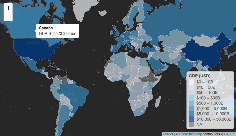

This chunk creates the interactive world map. Each country is colored by its GDP, with a color gradient applied according to the custom bins. The map includes interactive popups for each country and a customized legend that displays GDP in billions of US dollars.

Conclusion

We’ve demonstrated how to automate the generation of world map code using LLM-powered tools directly from R, preparing real datasets and joining them with geospatial data, and customizing your interactive leaflet map for your own use cases. This approach gives you full programmatic control, reproducibility, and the opportunity to adapt AI-generated code exactly how you want it.

Thank you for following this tutorial—experiment and customize further to make your own interactive world maps!

See you in another tutorial, bye bye!

Felix Analytix

Discussion about this post

Ready for more?